Extracting Water Body Footprint from Multispectral and Radar Imagery

INTRODUCTION

Readers of my earlier Remote Sensing posts (pre-2022), or any news article on the subject, typically encounter only the final output—processed satellite imagery accompanied by analysis or commentary. The processing chain itself is rarely shown. In a way, that makes sense: most people prefer admiring a finished painting, rather than watching an artist grind through the painstaking process of creation.

That said, those mesmerising time-lapse artistry videos on social media prove there is real joy in watching the process unfold—especially when it is condensed, structured and purposeful.

Processing satellite imagery is similar. It is exploratory by nature—almost like an archaeological dig, where peeling away each layer reveals something new.

In this post, you will see how satellite imagery is analysed to extract Water Body Footprints, through a step-by-step demonstration using both Multispectral and Radar. You’ll also get a feel for SNAP, a powerful and widely used satellite imagery analytics software.

The study area is a cross-section of the beautiful Masurian Lake District in northeastern Poland, known for its 2,000+ lakes.

Because plotting the exact contours of a water body using aerial photographs or topographic surveys is challenging and resource-intensive, satellite imagery is almost always preferred. A Water Body Footprint serves as a foundational dataset for:

• Flood Mapping

• Water Level Monitoring

• Tidal Studies

• River Course Mapping

• Glacial/Permafrost Studies

• Hydrological Modelling

---

SECTION HYPERLINKS:

• Extracting Water Body Footprint using Multispectral Satellite Imagery

• Extracting Water Body Footprint using Radar Satellite Imagery

• Comparing the Footprints from both modalities

---

Figure 1: Electromagnetic Spectrum Infographic. Source: EO College

Multispectral Satellite imagery is acquired passively—the satellite captures solar reflectance across multiple spectral bands i.e. ranges of wavelength (Sunlight constitutes energy waves from the Visible Light, Infrared and Ultraviolet portions of the Electromagnetic Spectrum).

Synthetic Aperture Radar (SAR) Satellite Imagery for Earth Observation purposes, by contrast, is acquired through active illumination - the satellite transmits pulses of microwaves (these lie at the higher frequency-end of the Radio spectrum as seen in Figure 1 above) and records the returning energy (backscatter). As a result, this mode of acquiring imagery is also known as Microwave Remote Sensing.

Each modality has unique advantages and limitations. While Multispectral Imaging responds primarily to the biogeochemical properties of the surface, Radar Imaging captures information related to the physical structure, temperature, and moisture content of the terrain. Moreover, unlike solar radiation—which cannot penetrate atmospheric constituents such as clouds or aerosols due to its shorter wavelengths—microwaves have much longer wavelengths and can bypass these obstructions with ease. This makes radar suitable for acquiring surface information at night, during cloudy or rainy conditions, and even in highly polluted environments.

Before I begin demonstrating the processing steps, it helps to understand that sourcing satellite imagery requires some basic know-how: having clarity about the imagery characteristics, the desired resolution, the timeline of acquisition, the geographic extent, and where or how to obtain the data (including the associated costs). For this study, I have used both Multispectral and Radar datasets acquired by ESA’s Copernicus Earth Observation satellites. These datasets are free for registered users, and the acquisition workflow is covered in the video tutorials referenced in this post.

---

Workflow 1: Extracting Water Body Footprint using Multispectral Satellite Imagery

Figure 2 - Cloud-corrected Sentinel-2 Multispectral Imagery over the Masurian Lake District in Poland (March 2018), visualized in Natural Color on SNAP.

Figure 3 - The same dataset being visualized in MSI False-Color Infrared mode

Visualizing Multispectral Imagery in different spectral band combinations helps reveal the underlying surface characteristics. For instance, the False-Color Infrared visualization in Figure 3 makes it easy to distinguish water bodies (blue) from vegetation (red).

Figure 4 - MSI Land/Water visualization (top-left) along with pre-processed Cloud, Snow, and Water masks.

Satellite imagery may be available either raw or pre-processed. When available, pre-processed imagery saves considerable time and computing resources. The three masks shown above identify snow, cloud, and water pixels as estimated by the satellite operator (ESA Copernicus). These masks help interpret the imagery more effectively and allow us to exclude pixels—particularly cloud and snow cover—that could distort our analysis.

Figure 5 - Resampled Multispectral Imagery (10 m resolution) visualized in MSI Land/Water RGB mode.

As with any analytical workflow, the dataset must be cleaned and organized before running the actual processing. Sentinel-2 imagery contains 13 spectral bands captured at three different spatial resolutions (10 m, 20 m and 60 m). However, several SNAP tools do not support multi-resolution products. Therefore, I have resampled the entire imagery dataset to 10 m resolution.

The resampled imagery—now uniform and ready for processing—is visualized above using the B2, B3, and B8 bands, all originally captured ar 10 m resolution).

Figure 6 - Output after Subset processing (Geographic and Band subset)

To optimize further, I removed components that are irrelevant for this workflow. Raw Sentinel-2 imagery can exceed 1 GB, and processing the entire dataset would be slow and resource-intensive. Subsetting allows us to:

Subset processing can involve-

• clip the geographic extent to the study area,

• retain only the required spectral bands, and

• optionally remove metadata layers not needed for analysis.

After applying both (1) Geographic Extent and (2) Band Subset, the dataset size dropped below 100 MB. With a clean, organized product, we can now begin extracting the Water Body Footprint.

---

Normalized Difference Water Index (NDWI)developed by S. K. McFeeters (1996), selectively amplifies the spectral response of water pixels, making it easier to delineate water bodies.

Figure 7: NDWI computation formula (McFeeters, 1996)

The formula is mathematically simple—just a normalized ratio of two spectral bands—but its conceptual basis rests on understanding how different surface types interact with electromagnetic radiation.

Sunlight, the illumination source for multispectral imagery, comprises visible, infrared, and ultraviolet energy. Water reflects visible light in amounts comparable to soil and vegetation, but when exposed to Near Infrared (NIR) wavelengths, water absorbs nearly all the energy and reflects none. Hence, in NIR, water pixels appear dark. Soil and vegetation, however, reflect NIR moderately, making those pixels appear bright. NDWI leverages this contrast in reflectance to identify water pixels.

 Reflectance properties of Water, Soil & Vegetation (Source: RUS Copernicus)

Amplifying this contrast is especially important when:

• water is shallow or turbid,

• the shoreline is mixed with urban structures, or

• background reflectance from nearby features interferes with water detection.

NDWI essentially checks whether a pixel’s NIR reflectance exceeds its Green reflectance:

• If NIR > Green, the NDWI becomes negative → Land

• If NIR < Green, the NDWI becomes positive → Water

This creates a simple and robust separation between water and land.

Figure 9 - NDWI (left) and Reclassified NDWI (right)

The image on the left shows the raw NDWI result:

• Bright pixels (0 to +1) → Water

• Dark pixels (0 to –1) → Land

To make the footprint extraction cleaner, I reclassified:

• all negative (land) values → NoData (black)

• all positive (water) values → 1 (white)

This binary mask allows us to extract a clean Water Footprint layer comparable with the Radar-derived footprint.

While NDWI is widely used, it also has limitations. Urban reflections and highly turbid water can create ambiguity. Several improved variants of NDWI exist (see pages 23-24 of this linked document) to address such challenges and improve water delineation across diverse landscapes.

---

Workflow 2: Extracting Water Body Footprint using Radar Satellite Imagery

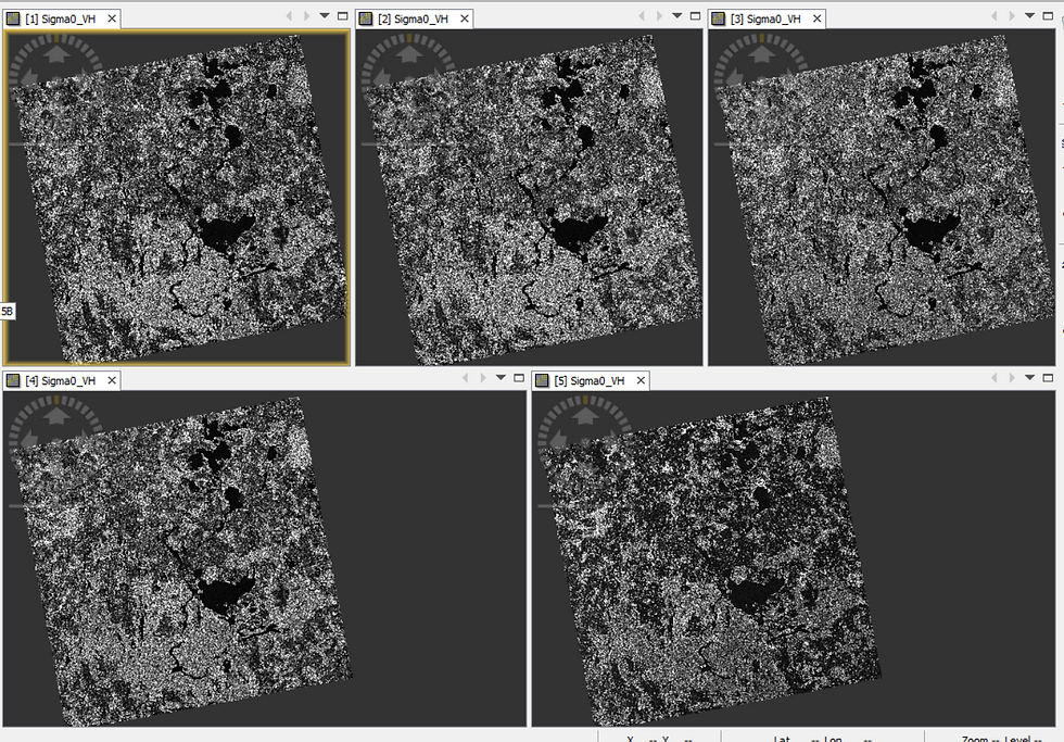
The workflow for extracting a Water Body Footprint from Radar Satellite Imagery differs markedly from the Multispectral approach. While the earlier workflow relied on a single Multispectral dataset, this Radar-based workflow uses five Sentinel-1 SAR datasets acquired between October and December 2020. The reason for using multiple datasets becomes clear later. Sentinel-1 Interferometric Wide-Swath (IW) imagery has a spatial resolution of 5 m × 20 m, meaning each pixel represents roughly 100 sq. m.

After applying a Geographic Extent subset (same extent as the Multispectral subset), a single raw Sentinel-1 scene looks like-

Figure 10 - Amplitude band of a raw Sentinel-1 Radar dataset (October 2020) over the Masurian Lake District, Poland

Although the scene appears as a scatter of salt-and-pepper pixels, the large water bodies are identifiable by the clusters of dark pixels.

Why are water pixels dark?

Because microwaves transmitted by the satellite strike water surfaces and are almost entirely reflected away from the sensor. Very little energy returns as backscatter, resulting in near-zero amplitude values, which appear black.

Conversely, vegetation, bare soil, and built-up features scatter microwaves back toward the sensor in moderate to high quantities, producing brighter pixels.

Figure 11 - Applying updated Orbit Files

The next pre-processing step is to apply the latest Orbit Files to all five scenes.

Orbit Files contain the satellite’s precise position and velocity during image acquisition. Accurate orbit metadata enables proper Geocoding—the assignment of backscatter values to the correct pixel locations. Since refined orbit solutions are generated a few days after acquisition, the default onboard values may be slightly inaccurate. Thus, updating to the latest Orbit Files is recommended.

Figure 12 - Pre (left) and Post (right) Thermal Noise Removal

The radar receiver generates its own background energy, known as thermal noise, which artificially inflates pixel intensities. This is undesirable in a classification workflow.

After applying Thermal Noise Removal, observe how certain pixels appear darker—this indicates that unwanted receiver noise has been removed.

Figure 13 - Pre (left) and Post (right) Radiometric Calibration

The next pre-processing step is to apply Radiometric Calibration to the Imagery dataset.

Radiometric Calibration converts the raw digital backscatter values into physically meaningful radiometric quantities measured at the Earth’s surface. It removes radiometric bias and applies offsets and other technical procedures required for accurate geocoding.

This step is essential for any analysis that compares multiple scenes pixel-to-pixel, which is critical for this Water Body Footprint workflow.

Figure 14 - Terrain-corrected Output

Next, I've applied another pre-processing step known as Terrain Correction.

Radar images are initially stored in satellite geometry i.e. in the orientation of how the satellite receives information in its orbit and not how the features appear on the surface of the earth in terms of distance between surface features and Arctic Circle (True North). As a result, the the distance and orientation relative to the Earth's surface is distorted.

Terrain Correction applies a map projection to reorient the imagery into proper geographic coordinates.

Map Projections is a comprehensive topic by itself so I'll not delve into that. However, do notice how the corrected output (Figure 14) is inverted and narrower than the raw image (Figure 10). This orientation matches how the Masurian Lake District appears on standard maps and also aligns with the Multispectral dataset (Figure 9).

To avoid repeating all of the above steps manually on each of the five scenes, I codified the workflow using SNAP’s Graph Builder and executed it on all datasets using Batch Processing.

Figure 15 - Processing chain defined in Graph Builder

Figure 16 - Batch Processing applied to all five Radar datasets

Figure 17 - All pre-processed datasets stacked side-by-side

The final pre-processing step is Coregistration. Since the five scenes are still treated as separate products, they must be aligned into a single multi-temporal stack, enabling pixel-level comparison.

Figure 18 — Coregistered stack visible in Product Explorer

Each dataset now appears as an individual band within a unified product, allowing further analysis via Band Maths.

This is where Einstein’s remark becomes fitting: If I had an hour to solve a problem, I’d spend fifty-five minutes understanding it and five minutes solving it.

The heavy lifting in this workflow lies in careful pre-processing; the actual analytics happen quickly thereafter.

---

Figure 19 - RGB visualization of a three-date Coregistered Stack

To deviate from the Water Footprint workflow slightly, Figure 19 above depicts a different Coregistered Stack comprising three of the five pre-processed imagery datasets visualized in RGB mode. While the rendered visualization appears like a natural-color photograph, it is actually a multi-temporal photograph through which one can observe the backscatter trend across the three acquisition dates:

• Black pixels — consistently no backscatter (likely water)

• Salt-and-pepper textures — fluctuating backscatter (vegetation or built-up areas)

• Green pixels — change between dates 1 and 2 (e.g., agricultural harvesting)

• Violet pixels — change between dates 2 and 3 (another harvest cycle)

This is a powerful way to visualize surface change from multiple dates in a single image!

---

To reduce noise further and stabilise pixel intensities, I computed the mean intensity at each pixel location across all five scenes, generating a sixth band. Averaging helps suppress residual speckle and intensity anomalies, enabling clearer delineation of water pixels in the next step.

Figure 20 - New averaged band (bottom-right), noticeably smoother

Figure 21 - Pixel Intensity of Coregistered Multi-temporal Radar Imagery Stack visualized using a Histogram

The final analysis step involves extracting the water pixels by thresholding the intensity values to demarcate it from land pixels.

However, notice from the histogram in Figure 21 that the land and water pixel values are still very close together. This makes the task of thresholding very challenging.

So, what’s the solution?

There is a very nifty way: amplifying the intensity values would allow for convenient thresholding.

In Figure 22 below, observe that the dark pixels on the left image appear darker on the right image and the bright pixels on the left image appear brighter on the right image-

Figure 22 - Log-scaled output (right) vs linear output (left)

What has happened here?

By applying a logarithmic transformation (dB = 10 × log10), the contrast between pixel values increases significantly:

• dark pixels become darker

• bright pixels become brighter

  
  

This separation enables cleaner classification.

Figure 23 - Histogram of log-scaled values (now bi-modal)

The histogram now displays two distinct peaks—one for water and one for land.

From the observed separation, pixels with log-scaled intensity < –23.54 dB represent water, and those above represent land.

Logarithms are useful after all!😁

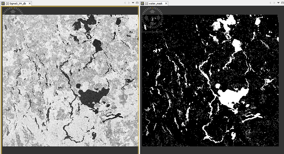
Using the –23.54 dB threshold in Band Maths:

• water pixels → assigned value 1

• land pixels → assigned NoData

This creates a binary mask identical in structure to the Multispectral NDWI output.

Figure 24 - Thresholded output (left) and reclassified Water Footprint (right)

---

Comparing the Footprints from both modalities

Lastly, let me show you how the two extracted Water Body Footprints, derived from processing Multispectral and Radar Satellite Imagery respectively, compare to each other-

Figure 25 - Merging both the extracted Water Body Footprint layers into a singular depiction

I have used GIS software to merge both the Footprints into a single Map view, as is depicted in Figure 25 above.

In the combined map:

• Violet pixels → identified as water by both workflows (majority)

• Red pixels → water only in Multispectral

• Blue pixels → water only in Radar

The extensive violet regions indicate strong consistency between the two methods.

Where discrepancies exist, the reasons typically involve:

a) Seasonal differences in acquisition Multispectral imagery was taken in spring, whereas Radar datasets were taken in autumn and winter. Water presence can legitimately differ.

b) Different sensing mechanisms Multispectral imaging uses passive sunlight; Radar uses active microwave illumination. Their responses, pre-processing steps, and limitations differ accordingly. Here's a comparison from the point-of-view of this Water Body Footprint extraction workflow in particular.

Do these footprints match ground-truth maps?

See for yourself-

Slider 1: Multispectral (O) and Radar (R) footprints overlaid on Google Maps

I hope you enjoyed exploring the satellite imagery analytics behind this workflow (something that I had promised at the outset😊)—just as much as the final result itself.

Thank you for reading!

---

ABOUT US - OPERATIONS MAPPING SOLUTIONS FOR ORGANIZATIONS

Intelloc Mapping Services, Kolkata | Mapmyops.com offers a suite of Mapping and Analytics solutions that seamlessly integrate with Operations Planning, Design, and Audit workflows. Our capabilities include — but are not limited to — Drone Services, Location Analytics & GIS Applications, Satellite Imagery Analytics, Supply Chain Network Design, Subsurface Mapping and Wastewater Treatment. Projects are executed pan-India, delivering actionable insights and operational efficiency across sectors.

My firm's services can be split into two categories - Geographic Mapping and Operations Mapping. Our range of offerings are listed in the infographic below-

Range of solutions that Intelloc Mapping Services (Mapmyops.com) offers

A majority of our Mapping for Operations-themed workflows (50+) can be accessed from this website's landing page. We respond well to documented queries/requirements. Demonstrations/PoC can be facilitated, on a paid-basis. Looking forward to being of service.

Regards,

Arpit Shah

Credits: EU Copernicus, RUS Copernicus & QGIS. Tutorial using older imagery can be viewed here.